¶Let  be a partition. The Young diagram of is the
array of boxes having
be a partition. The Young diagram of is the
array of boxes having  boxes in the
  -th row, left adjusted. Thus
if
-th row, left adjusted. Thus
if  the diagram is:
![\def\lr#1#2#3{\multicolumn{1}{#1@{\hspace{.6ex}}c@{\hspace{.6ex}}#2}{\raisebox{-.3ex}{$#3$}}}\raisebox{-6ex}{\begin{array}[b]{cccc}\cline{1-3}\lr{|}{|}{\;}&\lr{|}{|}{\;}&\lr{|}{|}{\;}\\ \cline{1-3}\lr{|}{|}{}&\lr{|}{|}{}&&\\ \cline{1-2}\end{array}}](_images/math/8888b2384babdfd89404d364d2c65a5cd0f9907c.png)
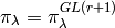
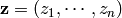
A semi-standard Young tableau of shape is a filling of the
box by integers in which the rows are weakly decreasing and the columns are
strictly decreasing. Thus
![\def\lr#1#2#3{\multicolumn{1}{#1@{\hspace{.6ex}}c@{\hspace{.6ex}}#2}{\raisebox{-.3ex}{$#3$}}}\raisebox{-6ex}{\begin{array}[b]{cccc}\cline{1-3}\lr{|}{|}{3}&\lr{|}{|}{2}&\lr{|}{|}{2}\\ \cline{1-3}\lr{|}{|}{2}&\lr{|}{|}{1}&&\\ \cline{1-2}\end{array}}](_images/math/b16fc8dcb8f20b794e615033a6e6b89c7c53254d.png)
is a semistandard Young tableau. Sage has a Tableau class, and you may create this tableau as follows:
sage: T=Tableau([[3,2,2],[2,1]]); T
[[3, 2, 2], [2, 1]]
A partition of length  is a dominant weight for
  according
to the description of the ambient space in Standard realizations of the ambient spaces. Therefore
it corresponds to an irreducible representation
according
to the description of the ambient space in Standard realizations of the ambient spaces. Therefore
it corresponds to an irreducible representation
 of .
of .
It is true that not every dominant weight is a partition, since a
dominant weight might have some values negative. The dominant
weight is a partition if and only if the character of
is a polynomial as a function on the space  .
Thus for example
.
Thus for example  with
with 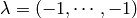 ,
which is a dominant weight but not a partition, and the character is not
a polynomial function on
,
which is a dominant weight but not a partition, and the character is not
a polynomial function on
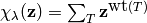
Theorem (Littlewood) If is a partition, then the number of Semi-Standard Young
Tableaux with shape and entries in 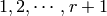 is the dimension
of
is the dimension
of  .
.
For example, if  and
and  , then we find 15 tableaux with shape and entries in
  :
:
![\begin{array}{ccccc}{\def\lr#1{\multicolumn{1}{|@{\hspace{.6ex}}c@{\hspace{.6ex}}|}{\raisebox{-.3ex}{$#1$}}}\raisebox{-.6ex}{$\begin{array}[b]{ccc}\cline{1-1}\cline{2-2}\cline{3-3}\lr{1}&\lr{1}&\lr{1}\\\cline{1-1}\cline{2-2}\cline{3-3}\lr{2}&\lr{2}\\\cline{1-1}\cline{2-2}\end{array}$}}&{\def\lr#1{\multicolumn{1}{|@{\hspace{.6ex}}c@{\hspace{.6ex}}|}{\raisebox{-.3ex}{$#1$}}}\raisebox{-.6ex}{$\begin{array}[b]{ccc}\cline{1-1}\cline{2-2}\cline{3-3}\lr{1}&\lr{1}&\lr{2}\\\cline{1-1}\cline{2-2}\cline{3-3}\lr{2}&\lr{2}\\\cline{1-1}\cline{2-2}\end{array}$}}&{\def\lr#1{\multicolumn{1}{|@{\hspace{.6ex}}c@{\hspace{.6ex}}|}{\raisebox{-.3ex}{$#1$}}}\raisebox{-.6ex}{$\begin{array}[b]{ccc}\cline{1-1}\cline{2-2}\cline{3-3}\lr{1}&\lr{1}&\lr{3}\\\cline{1-1}\cline{2-2}\cline{3-3}\lr{2}&\lr{2}\\\cline{1-1}\cline{2-2}\end{array}$}}&{\def\lr#1{\multicolumn{1}{|@{\hspace{.6ex}}c@{\hspace{.6ex}}|}{\raisebox{-.3ex}{$#1$}}}\raisebox{-.6ex}{$\begin{array}[b]{ccc}\cline{1-1}\cline{2-2}\cline{3-3}\lr{1}&\lr{1}&\lr{3}\\\cline{1-1}\cline{2-2}\cline{3-3}\lr{2}&\lr{3}\\\cline{1-1}\cline{2-2}\end{array}$}}&{\def\lr#1{\multicolumn{1}{|@{\hspace{.6ex}}c@{\hspace{.6ex}}|}{\raisebox{-.3ex}{$#1$}}}\raisebox{-.6ex}{$\begin{array}[b]{ccc}\cline{1-1}\cline{2-2}\cline{3-3}\lr{1}&\lr{2}&\lr{3}\\\cline{1-1}\cline{2-2}\cline{3-3}\lr{2}&\lr{3}\\\cline{1-1}\cline{2-2}\end{array}$}}\\\\{\def\lr#1{\multicolumn{1}{|@{\hspace{.6ex}}c@{\hspace{.6ex}}|}{\raisebox{-.3ex}{$#1$}}}\raisebox{-.6ex}{$\begin{array}[b]{ccc}\cline{1-1}\cline{2-2}\cline{3-3}\lr{1}&\lr{1}&\lr{3}\\\cline{1-1}\cline{2-2}\cline{3-3}\lr{3}&\lr{3}\\\cline{1-1}\cline{2-2}\end{array}$}}&{\def\lr#1{\multicolumn{1}{|@{\hspace{.6ex}}c@{\hspace{.6ex}}|}{\raisebox{-.3ex}{$#1$}}}\raisebox{-.6ex}{$\begin{array}[b]{ccc}\cline{1-1}\cline{2-2}\cline{3-3}\lr{1}&\lr{2}&\lr{3}\\\cline{1-1}\cline{2-2}\cline{3-3}\lr{3}&\lr{3}\\\cline{1-1}\cline{2-2}\end{array}$}}&{\def\lr#1{\multicolumn{1}{|@{\hspace{.6ex}}c@{\hspace{.6ex}}|}{\raisebox{-.3ex}{$#1$}}}\raisebox{-.6ex}{$\begin{array}[b]{ccc}\cline{1-1}\cline{2-2}\cline{3-3}\lr{2}&\lr{2}&\lr{3}\\\cline{1-1}\cline{2-2}\cline{3-3}\lr{3}&\lr{3}\\\cline{1-1}\cline{2-2}\end{array}$}}&{\def\lr#1{\multicolumn{1}{|@{\hspace{.6ex}}c@{\hspace{.6ex}}|}{\raisebox{-.3ex}{$#1$}}}\raisebox{-.6ex}{$\begin{array}[b]{ccc}\cline{1-1}\cline{2-2}\cline{3-3}\lr{1}&\lr{1}&\lr{1}\\\cline{1-1}\cline{2-2}\cline{3-3}\lr{2}&\lr{3}\\\cline{1-1}\cline{2-2}\end{array}$}}&{\def\lr#1{\multicolumn{1}{|@{\hspace{.6ex}}c@{\hspace{.6ex}}|}{\raisebox{-.3ex}{$#1$}}}\raisebox{-.6ex}{$\begin{array}[b]{ccc}\cline{1-1}\cline{2-2}\cline{3-3}\lr{1}&\lr{1}&\lr{2}\\\cline{1-1}\cline{2-2}\cline{3-3}\lr{2}&\lr{3}\\\cline{1-1}\cline{2-2}\end{array}$}}\\\\{\def\lr#1{\multicolumn{1}{|@{\hspace{.6ex}}c@{\hspace{.6ex}}|}{\raisebox{-.3ex}{$#1$}}}\raisebox{-.6ex}{$\begin{array}[b]{ccc}\cline{1-1}\cline{2-2}\cline{3-3}\lr{1}&\lr{2}&\lr{2}\\\cline{1-1}\cline{2-2}\cline{3-3}\lr{2}&\lr{3}\\\cline{1-1}\cline{2-2}\end{array}$}}&{\def\lr#1{\multicolumn{1}{|@{\hspace{.6ex}}c@{\hspace{.6ex}}|}{\raisebox{-.3ex}{$#1$}}}\raisebox{-.6ex}{$\begin{array}[b]{ccc}\cline{1-1}\cline{2-2}\cline{3-3}\lr{1}&\lr{1}&\lr{1}\\\cline{1-1}\cline{2-2}\cline{3-3}\lr{3}&\lr{3}\\\cline{1-1}\cline{2-2}\end{array}$}}&{\def\lr#1{\multicolumn{1}{|@{\hspace{.6ex}}c@{\hspace{.6ex}}|}{\raisebox{-.3ex}{$#1$}}}\raisebox{-.6ex}{$\begin{array}[b]{ccc}\cline{1-1}\cline{2-2}\cline{3-3}\lr{1}&\lr{1}&\lr{2}\\\cline{1-1}\cline{2-2}\cline{3-3}\lr{3}&\lr{3}\\\cline{1-1}\cline{2-2}\end{array}$}}&{\def\lr#1{\multicolumn{1}{|@{\hspace{.6ex}}c@{\hspace{.6ex}}|}{\raisebox{-.3ex}{$#1$}}}\raisebox{-.6ex}{$\begin{array}[b]{ccc}\cline{1-1}\cline{2-2}\cline{3-3}\lr{1}&\lr{2}&\lr{2}\\\cline{1-1}\cline{2-2}\cline{3-3}\lr{3}&\lr{3}\\\cline{1-1}\cline{2-2}\end{array}$}}&{\def\lr#1{\multicolumn{1}{|@{\hspace{.6ex}}c@{\hspace{.6ex}}|}{\raisebox{-.3ex}{$#1$}}}\raisebox{-.6ex}{$\begin{array}[b]{ccc}\cline{1-1}\cline{2-2}\cline{3-3}\lr{2}&\lr{2}&\lr{2}\\\cline{1-1}\cline{2-2}\cline{3-3}\lr{3}&\lr{3}\\\cline{1-1}\cline{2-2}\end{array}$}}\end{array}](_images/math/f0d9d736f947c185d9640cbf94b514c4f4aadc82.png)
This is consistent with the theorem since the dimension of the irreducible
representation of  with highest weight
  has dimension 15:
sage: A2=WeylCharacterRing("A2")
sage: A2(3,2,0).degree()
15
In fact we may obtain the character of the representation from the set of tableaux.
Indeed, one of the definitions of the Schur polynomial (due to Littlewood) is
the following combinatorial one. If  is a tableaux, define the
weight of to be
is a tableaux, define the
weight of to be 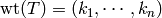 where
where
 is the number of ‘s in the tableaux. Then the
multiplicity of
is the number of ‘s in the tableaux. Then the
multiplicity of  in the character
  is the
number of tableaux of weight . Thus if
is the
number of tableaux of weight . Thus if
 , we have
where the sum is over all semistandard Young tableaux of shape
that have entries in .
¶Representations of the symmetric group are parametrized by partitions
of  . The parametrization may be characterized as follows.
Let
. The parametrization may be characterized as follows.
Let  be any integer
  . Then both
  and
act on
and
act on  where
where  . Indeed, acts on
each
. Indeed, acts on
each  and permutes them. Then if
  is the
representation of with highest weight vector
and
is the
representation of with highest weight vector
and  is the irreducible representation of
parametrized by then
is the irreducible representation of
parametrized by then
as bimodules for the two groups. This is Frobenius-Schur duality and
it serves to characterize the parametrization of the irreducible
representations of by partitions of .
Let us say that a Tableaux of shape  is standard
if contains each entry
is standard
if contains each entry  exactly once.
Theorem (Young, 1927) The degree of is the number of standard
tableaux of shape .
References:
The Robinson-Schensted-Knuth correspondence gives bijections between pairs of tableaux of various types and combinatorial objects of different types. We will not review the correspondence in detail here, but see the references. We note that Schensted insertion is implemented as the method schensted_insertion() of Tableau class in Sage.
Thus we have the following bijections:
as runs through the partitions of are in bijection
with the  elements of .
 and
and  of shape where
runs through the partitions of such that
is a standard tableau and is a semistandard tableau in
of shape where
runs through the partitions of such that
is a standard tableau and is a semistandard tableau in
 are in bijection with the
  words of
length in . and of the same shape but
arbitrary size in
words of
length in . and of the same shape but
arbitrary size in  are in bijection with
  positive integer matrices. and of conjugate shapes
and
positive integer matrices. and of conjugate shapes
and  are in bijection with
matrices with entries
are in bijection with
matrices with entries  or
or  .
.The three bijections cited above have the following analogs in representation theory.
 is an
is an  bimodule
with of dimension . It decomposes as a direct sum of
bimodule
with of dimension . It decomposes as a direct sum of
 .-dimensional vector space
  where
where  into the direct sum of
  as a bimodule, where runs through partitions of .
 on which
  acts by
  . The polynomial ring
decomposes into the direct sum of
. The polynomial ring
decomposes into the direct sum of  .
Taking traces gives the Cauchy identity.. Taking traces gives the dual
Cauchy identity.
.
Taking traces gives the Cauchy identity.. Taking traces gives the dual
Cauchy identity.The theory of quantum groups interpolates between the representation
theoretic picture and the combinatorial picture, and thereby
explains these analogies. The representation
is reinterpreted as a module for the quantized enveloping algebra
 , and the representation
is reinterpreted as a module for the Iwahori
Hecke algebra. Then Frobenius-Schur duality persists. Reference:
, and the representation
is reinterpreted as a module for the Iwahori
Hecke algebra. Then Frobenius-Schur duality persists. Reference:
 -analogue of
  , Hecke algebra,
and the Yang-Baxter equation. Lett. Math. Phys. 11 (1986), no. 3, 247–252.
, Hecke algebra,
and the Yang-Baxter equation. Lett. Math. Phys. 11 (1986), no. 3, 247–252.When  , we recover the representation story. When
  ,
we recover the combinatorial story.
,
we recover the combinatorial story.
References:
-analogue of classical Lie algebras. J. Algebra 165 (1994), no. 2,
295–345.Kashiwara considered the highest weight modules of quantized enveloping
algebras  in the limit when . The enveloping
algebra cannot be defined when
in the limit when . The enveloping
algebra cannot be defined when  , but a limiting structure can still be
detected. This is the crystal basis of the module.
, but a limiting structure can still be
detected. This is the crystal basis of the module.
Kashiwara’s crystal bases have a combinatorial structure that sheds light even on purely combinatorial constructions on tableaux that predated quantum groups. It gives a good generalization to other Cartan types.
We will not make the most general definition of a crystal. See the references
for a more general definition. Let  be the weight lattice of a classical
Cartan type.
be the weight lattice of a classical
Cartan type.
We now define a crystal of type  . Let
. Let  be a set,
and let
be a set,
and let  be an auxiliary element. For each index
  we assume there given maps
  , maps
  and a map
 satisfying certain
assumptions, which we now describe.
It is assumed that if
satisfying certain
assumptions, which we now describe.
It is assumed that if  then
then  if and only if
  . In this case, it
is assumed that
. In this case, it
is assumed that

Moreover, we assume that

for all  .
.
Assumption (Regularity) We will assume that  is the
number of times that
is the
number of times that  may applied to
  , and that
  is the
number of times that
is the
number of times that  may be applied. That is,
 and
and 
This regularity assumption is not made by Kashiwara, but it is satisfied by the
crystals that we are concerned with here. Kashiwara also allows  and
and  to take the value
  .
.
Given the crystal , the character  is:
is:
 .
.
Given any highest weight , constructions of Kashiwara and Nakashima,
Littelmann and others produce a crystal  such that
 , where is the irreducible
character with highest weight , as in Representations and Characters.
, where is the irreducible
character with highest weight , as in Representations and Characters.
The crystal  is not uniquely characterized by the
properties that we have stated so far. For Cartan types A,D,E it may
be characterized by these properties together with certain other
Stembridge axioms. We will take it for granted that there is a
unique “correct” crystal and discuss how these
are constructed in Sage.
is not uniquely characterized by the
properties that we have stated so far. For Cartan types A,D,E it may
be characterized by these properties together with certain other
Stembridge axioms. We will take it for granted that there is a
unique “correct” crystal and discuss how these
are constructed in Sage.
Before giving examples of crystals, we digress to help you install dot2tex, which you will need in order to make latex images of crystals.
You may download the following file:
http://sage.math.washington.edu/home/nthiery/dot2tex-2.8.7.spkg
Then run:
sage -i dot2tex-2.8.7.spkg
to install the package.
For type  , Kashiwara and Nakashima put a crystal
structure on the set of tableaux with shape
in
, Kashiwara and Nakashima put a crystal
structure on the set of tableaux with shape
in  , and this is a realization of
. Moreover, this construction extends
to other Cartan types, as we will explain. At the moment, we will
consider how to draw pictures of these crystals.
, and this is a realization of
. Moreover, this construction extends
to other Cartan types, as we will explain. At the moment, we will
consider how to draw pictures of these crystals.
Once you have dot2tex installed, you may make images pictures of crystals as follows:
sage: C=CrystalOfTableaux("A2",shape=[2,1])
sage: C.latex_file("/tmp/a2rho.tex")
Here 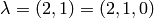 . The crystal C is
  .
The character will therefore be the eight-dimensional irreducible
character with this highest weight. The method latex_file() produces
.
The character will therefore be the eight-dimensional irreducible
character with this highest weight. The method latex_file() produces
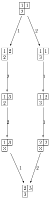
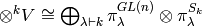
As you can see, the elements of this crystal are exactly the eight tableaux
of shape with entries in . The convention is that if
 and
and  , or equivalently
  , then we
draw an arrow from
, then we
draw an arrow from  . Thus the highest weight tableau is the
one with no incoming arrows. Indeed, this is:
. Thus the highest weight tableau is the
one with no incoming arrows. Indeed, this is:
![{\def\lr#1{\multicolumn{1}{|@{\hspace{.6ex}}c@{\hspace{.6ex}}|}{\raisebox{-.3ex}{$#1$}}}\raisebox{-.6ex}{$\begin{array}[b]{ccc}\cline{1-1}\cline{2-2}\lr{1}&\lr{1}\\\cline{1-1}\cline{2-2}\lr{2}\\\cline{1-1}\end{array}$}}](_images/math/e1c44d83cf8259bfecf9b8196308399679273f03.png)
We recall that the weight of the tableau is  where is the number of
‘s in the tableau, so this tableau has weight
where is the number of
‘s in the tableau, so this tableau has weight  , which indeed equals .
Once the crystal is created, you have access to the ambient space and its methods through the method :meth:weight_lattice_realization():
sage: L = C.weight_lattice_realization(); L
Ambient space of the Root system of type ['A', 2]
sage: L.fundamental_weights()
Finite family {1: (1, 0, 0), 2: (1, 1, 0)}
The highest weight vector is available as follows:
sage: v = C.highest_weight_vector(); v
[[1, 1], [2]]
or more simply:
sage: C[0]
[[1, 1], [2]]
Now we may apply the operators and to
move around in the crystal:
sage: v.f(1)
[[1, 2], [2]]
sage: v.f(1).f(1)
sage: v.f(1).f(1) == None
True
sage: v.f(1).f(2)
[[1, 3], [2]]
sage: v.f(1).f(2).f(2)
[[1, 3], [3]]
sage: v.f(1).f(2).f(2).f(1)
[[2, 3], [3]]
sage: v.f(1).f(2).f(2).f(1) == v.f(2).f(1).f(1).f(2)
True
You can construct the character if you first make a Weyl character ring:
sage: A2 = WeylCharacterRing("A2")
sage: C.character(A2)
A2(2,1,0)
For each of the classical Cartan types there is a standard
crystal  from which other
crystals can be built up by taking tensor products and extracting
constituent irreducible crystals. This procedure is sufficient
for Cartan types and
from which other
crystals can be built up by taking tensor products and extracting
constituent irreducible crystals. This procedure is sufficient
for Cartan types and  . For types
  and
and  the standard crystal must be supplemented with a spin crystal.
The crystal of letters is a special case of the crystal of tableaux
in the sense that is isomorphic
the crystal of tableaux whose highest weight is the
highest weight vector of the standard representation. Thus compare:
sage: CrystalOfLetters("A3")
The crystal of letters for type ['A', 3]
sage: CrystalOfTableaux("A3",shape=[1])
The crystal of tableaux of type ['A', 3] and shape(s) [[1]]
These two crystals are different in implementation, but they are isomorphic, and in fact the second crystal is constructed from the first. Crystals of letters have a special role in the theory since they are particularly simple, yet as Kashiwara and Nakashima showed, the crystals of tableaux can be created from them. We will review how this works.
Kashiwara defined the tensor product of crystals in a purely combinatorial
way. The beauty of this construction is that it exactly parallels the
tensor product of crystals of representations. That is, if
and are dominant weights, then
 is a (usually
disconnected) crystal which may contain multiple copies of
is a (usually
disconnected) crystal which may contain multiple copies of
 (for another dominant weight
  ) but the
number of copies of is exactly the multiplicity
of
) but the
number of copies of is exactly the multiplicity
of  in
in  .
.
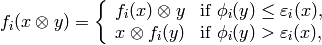
We will describe two conventions for the tensor product of crystals. These conventions would have to be modified slightly without the regularity assumption.
As a set, the tensor product  of crystals
and
of crystals
and  is the Cartesian product, but we denote the
ordered pair
is the Cartesian product, but we denote the
ordered pair  with and
  by
by  . We define
  . We define
and
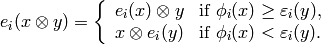
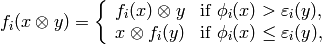
It is understood that 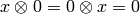 . We also define:


As a set, the tensor product of crystals
and is the Cartesian product, but we denote the
ordered pair  with
with  and
and  by . We define
  . We define
and
It is understood that  . We also define


The tensor product is associative:  is
an isomorphism
is
an isomorphism  ,
and so we may consider tensor products of arbitrary numbers of crystals.
,
and so we may consider tensor products of arbitrary numbers of crystals.
The relationship between the two definitions is simply that the
Kashiwara tensor product  is the
alternate tensor product
is the
alternate tensor product  in
reverse order. Sage uses the alternative tensor product. Even
though the tensor product construction is a priori asymmetrical,
both constructions produce isomorphic crystals, and in particular Sage’s
crystals of tableaux are identical to Kashiwara’s.
in
reverse order. Sage uses the alternative tensor product. Even
though the tensor product construction is a priori asymmetrical,
both constructions produce isomorphic crystals, and in particular Sage’s
crystals of tableaux are identical to Kashiwara’s.
You may construct the tensor product of several crystals in Sage using TensorProductOfCrystals:
sage: C = CrystalOfLetters("A2")
sage: T = TensorProductOfCrystals(C,C,C); T
Full tensor product of the crystals [The crystal of letters for type ['A', 2],
The crystal of letters for type ['A', 2], The crystal of letters for type ['A', 2]]
sage: T.cardinality()
27
sage: T.highest_weight_vectors()
[[1, 1, 1], [1, 2, 1], [2, 1, 1], [3, 2, 1]]
This crystal has four highest weight vectors. We may understand this as follows:
sage: A2 = WeylCharacterRing("A2")
sage: chi_C = C.character(A2)
sage: chi_T = T.character(A2)
sage: chi_C
A2(1,0,0)
sage: chi_T
A2(1,1,1) + 2*A2(2,1,0) + A2(3,0,0)
sage: chi_T == chi_C^3
True
As expected, the character of T is the cube of the character of C, and
representations with highest weight  ,
,  and . This
decomposition is predicted by Frobenius-Schur duality: the multiplicity
of in
and . This
decomposition is predicted by Frobenius-Schur duality: the multiplicity
of in  is the degree of
of
is the degree of
of  .
.
It is useful to be able to select one irreducible constitutent of T. If we only want one of the irreducible constituents of T, we can specify a list of highest weight vectors by the option generators. If the list has only one element, then we get an irreducible crystal. We can make four such crystals:
sage: [T1,T2,T3,T4] = \
[TensorProductOfCrystals(C,C,C,generators=[v]) for v in T.highest_weight_vectors()]
sage: [B.cardinality() for B in [T1,T2,T3,T4]]
[10, 8, 8, 1]
sage: [B.character(A2) for B in [T1,T2,T3,T4]]
[A2(3,0,0), A2(2,1,0), A2(2,1,0), A2(1,1,1)]
We see that two of these crystals are isomorphic, with character A2(2,1,0). Try:
sage: T1.plot(), T2.plot(), T3.plot(), T4.plot()
Elements of TensorProductOfCrystals(A,B,C, ...) are represented by
sequences [a,b,c, ...] with a in A, b in B, etc.
This of course represents  .
.
Sage implements the CrystalOfTableaux as a subcrystal of a tensor product of the CrystalOfLetters. You can see how its done as follows:
sage: T = CrystalOfTableaux("A3",shape=[3,1])
sage: v = T.highest_weight_vector().f(1).f(2).f(3).f(1).f(2); v
[[1, 3, 4], [2]]
sage: v._list
[2, 1, 3, 4]
We’ve looked at the internal representation of , where it is represented
as an element of the fourth tensor power of the CrystalOfLetters. We see that
the tableau:
![{\def\lr#1{\multicolumn{1}{|@{\hspace{.6ex}}c@{\hspace{.6ex}}|}{\raisebox{-.3ex}{$#1$}}}\raisebox{-.6ex}{$\begin{array}[b]{ccc}\cline{1-1}\cline{2-2}\cline{3-3}\lr{1}&\lr{3}&\lr{4}\\\cline{1-1}\cline{2-2}\cline{3-3}\lr{2}\\\cline{1-1}\end{array}$}}](_images/math/1536687e4bafcabfcf47aec38b21f8db9983ba15.png)
is interpreted as the tensor:
The elements of the tableau are read from bottom to top and from left to right. This is the inverse middle-Eastern reading of the tableau. See Hong and Kang, loc. cit. for discussion of the readings of a tableau.
For the Cartan types , or  , CrystalOfTableaux are capable of making any
finite crystal. (For type it is necessary that the highest weight be
a partition.)
, CrystalOfTableaux are capable of making any
finite crystal. (For type it is necessary that the highest weight be
a partition.)
For Cartan types and , CrystalOfTableaux fail to make
if is half-integral. For type  you can do this:
sage: B = FastCrystal(['B',2],shape=[3/2,1/2]); B
The fast crystal for B2 with shape [3/2,1/2]
sage: v = B.highest_weight_vector(); v.weight()
(3/2, 1/2)
However FastCrystals are only available for rank two Cartan types. We therefore have to do something else to create crystals of half-integral weight.
For types and the solution to this problem involves the use of
spin crystals.
The spin crystal has highest weight  . This is
the last fundamental weight. The irreducible representation with this weight
is the spin representation of degree
. This is
the last fundamental weight. The irreducible representation with this weight
is the spin representation of degree  . Its crystal is hand-coded in
Sage:
. Its crystal is hand-coded in
Sage:
sage: Cspin = CrystalOfSpins("B3"); Cspin
The crystal of spins for type ['B', 3]
sage: Cspin.cardinality()
8
We can make use of this to construct an arbitrary crystal with
highest weight , where is a half-integral
weight. For example, suppose that  . The
corresponding irreducible character will have degree 112:
. The
corresponding irreducible character will have degree 112:
sage: B3=WeylCharacterRing("B3")
sage: B3(3/2,3/2,1/2).degree()
112
So will have 112 elements. We can
find it as a subcrystal of Cspin ,
where
,
where  :
:
sage: B3(1,1,0)*B3(1/2,1/2,1/2)
B3(1/2,1/2,1/2) + B3(3/2,1/2,1/2) + B3(3/2,3/2,1/2)
We see that just taking the tensor product of these two crystals will produce a reducible crystal with three constitutents, and we want to extract the one we want. We do that as follows:
sage: C1 = CrystalOfTableaux("B3",shape=[1,1])
sage: C = TensorProductOfCrystals(C1,Cspin,generators=[[C1[0],Cspin[0]]])
sage: C.cardinality()
112
This is the desired crystal.
A similar situation pertains for type , but now there are two spin crystals,
both of degree  . These are hand-coded in sage:
sage: SpinPlus = CrystalOfSpinsPlus("D4")
sage: SpinMinus = CrystalOfSpinsMinus("D4")
sage: SpinPlus[0].weight()
(1/2, 1/2, 1/2, 1/2)
sage: SpinMinus[0].weight()
(1/2, 1/2, 1/2, -1/2)
sage: [C.cardinality() for C in [SpinPlus,SpinMinus]]
[8, 8]
You can use them similarly to the type B crystal of spins in order to construct any crystal of half-integral weight.
Let  be a Lie group and
  a Levi subgroup. We have already seen
that the Dynkin diagram of is obtained from that of by erasing
one or more nodes.
a Levi subgroup. We have already seen
that the Dynkin diagram of is obtained from that of by erasing
one or more nodes.
If is a crystal for , then we may obtain the corresponding
crystal for by a similar process. For example if the Dynkin-diagram
for is obtained from the Dynkin diagram for by erasing the -th
node, then if we erase all the edges in the crystal that
are labeled with , we obtain a crystal for .
Sage contains support for affine crystals. These lie outside the scope of this document.
Weyl Groups, Coxeter Groups and the Bruhat Order
