Since we must be brief here, this is not really a place to learn about Lie groups. Rather, the point of this section is to outline what you need to know to use Sage effectively for Lie computations, and to fix ideas and notations.
If  , then g may be uniquely factored as
 where
where  and
and  commute, with
semisimple (diagonalizable) and unipotent (all its eigenvalues
equal to 1). This follows from the Jordan canonical form. If
commute, with
semisimple (diagonalizable) and unipotent (all its eigenvalues
equal to 1). This follows from the Jordan canonical form. If  then
then
 is called semisimple and if
  then is
called unipotent.
then is
called unipotent.
We consider a Lie group  and a class of representations such that if
an element
and a class of representations such that if
an element  is unipotent (resp. semisimple) in one faithful
representation from the class, then it is unipotent (resp. semisimple) in
every faithful representation of the class. Thus the notion of being
semisimple or unipotent is intrinsic. Examples:
is unipotent (resp. semisimple) in one faithful
representation from the class, then it is unipotent (resp. semisimple) in
every faithful representation of the class. Thus the notion of being
semisimple or unipotent is intrinsic. Examples:
 with algebraic representations.
A subgroup of is called unipotent if it is connected and all its
elements are unipotent. It is called a torus if it is connected, abelian,
and all its elements are semisimple. The group is called reductive
if it has no nontrivial normal unipotent subgroup. For example,
 is reductive, but its subgroup:
is not since it has a normal unipotent subgroup
A group has a unique largest normal unipotent subgroup, called the unipotent radical, so it is reductive if and only if the unipotent radical is trivial.
A Lie group is called semisimple it is reductive and furthermore has no
nontrivial normal tori. For example is reductive but
not semisimple because it has a normal torus:
The group  is semisimple.
If is a semisimple Lie group then its center and fundamental group
are finite abelian groups. The universal covering group  is
therefore a finite extension with the same Lie algebra. Any representation of
may be reinterpreted as a representation of the simply connected
. Therefore we may as well consider representations of
, and restrict ourselves to the simply connected group.
is
therefore a finite extension with the same Lie algebra. Any representation of
may be reinterpreted as a representation of the simply connected
. Therefore we may as well consider representations of
, and restrict ourselves to the simply connected group.
Let be a reductive complex analytic group. A maximal solvable
subgroup of is called a Borel subgroup. All Borel subgroups are
conjugate. Any subgroup  containing a Borel subgroup is called a
parabolic subgroup. We may write as a semidirect product of its
maximal normal unipotent subgroup or unipotent radical and a
reductive subgroup
containing a Borel subgroup is called a
parabolic subgroup. We may write as a semidirect product of its
maximal normal unipotent subgroup or unipotent radical and a
reductive subgroup  , which is determined up to conjugacy. The
subgroup is called a Levi subgroup.
, which is determined up to conjugacy. The
subgroup is called a Levi subgroup.
Example: Let  and let
  be integers
whose sum is
be integers
whose sum is  . Then we may consider matrices of the form:
 ,
,
where 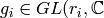 . The unipotent radical consists of the subgroup in
which all
. The unipotent radical consists of the subgroup in
which all  . The Levi subgroup (determined up to conjugacy) is:
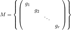 ,
,
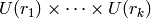
and is isomorphic to  . Therefore
is a Levi subgroup.
. Therefore
is a Levi subgroup.
The notion of a Levi subgroup can be extended to compact Lie groups. Thus
 is a Levi subgroup of
  . However
Parabolic subgroups do not exist for compact Lie groups.
. However
Parabolic subgroups do not exist for compact Lie groups.
Semisimple Lie groups are classified by their Cartan types. There
are both reducible and irreducible Cartan types in Sage. Let us
start with the irreducible types. Such a type is
implemented in Sage as a pair [`X`,r] where X is one of
A, B, C, D, E, F or G and  is a positive integer.
If X=D then we must have
is a positive integer.
If X=D then we must have  and if X is one of the
exceptional types
and if X is one of the
exceptional types  ,
,  or then is limited to only
a few possibilities. The exceptional types are:
or then is limited to only
a few possibilities. The exceptional types are:
['G',2], ['F',4], ['E',6], ['E',7] or ['E',8].
A simply-connected semisimple group is a direct product of simple Lie groups,
which are given by the following table. The integer is called the
rank, and is the dimension of the maximal torus.
Here are the Lie groups corresponding to the classical types:
| compact group | complex analytic group | Cartan type |
|---|---|---|
 |
 |
 |
 |
 |
 |
 |
 |
 |
 |
 |
 |
You may create these Cartan types and their Dynkin diagrams as follows:
sage: ct = CartanType("D5"); ct
['D', 5]
Here "D5" is an abbreviation for ['D',5].
Every Cartan type has a dual, which you can get from within Sage:
sage: CartanType("B4").dual()
['C', 4]
Types other than B and C are self-dual in the sense that the dual is isomorphic to the original type, but the isomorphism of a Cartan type with its dual might relabel the vertices. We can see this as follows:
sage: CartanType("F4").dynkin_diagram()
O---O=>=O---O
1   2   3   4
F4
sage: CartanType("F4").dual()
['F', 4]^*
sage: CartanType("F4").dual().dynkin_diagram()
O---O=<=O---O
1   2   3   4
F4*
If is a Lie group of finite index in  , where
  and
and
 are Lie groups of dimension
  , then is called reducible. In
this case, the root system of is the disjoint union of the root systems of
and , which lie in orthogonal subspaces of the ambient space of the
weight space of . The Cartan type of is thus reducible.
, then is called reducible. In
this case, the root system of is the disjoint union of the root systems of
and , which lie in orthogonal subspaces of the ambient space of the
weight space of . The Cartan type of is thus reducible.
Reducible Cartan types are supported in Sage as follows:
sage: RootSystem("A1xA1")
Root system of type A1xA1
sage: WeylCharacterRing("A1xA1")
The Weyl Character Ring of Type A1xA1 with Integer Ring coefficients
There are some isomorphisms that occur in low degree.
| Cartan Type | Group | Equivalent Type | Isomorphic Group |
|---|---|---|---|
| B2 |  |
C2 |  |
| D3 |  |
A3 |  |
| D2 |  |
A1xA1 |  |
| B1 |  |
A1 |  |
| C1 |  |
A1 | |
Sometimes the redundant Cartan types such as D3 and D2 are excluded
from the list of Cartan types. Folks will tell there’s no such Cartan
types. However Sage allows them since excluding them leads to exceptions
having to be made in algorithms. A better approach, which is followed by Sage,
is to allow the redundant Cartan types, but to implement the isomorphisms
explicitly as special cases of branching rules. The utility of this
approach may be seen by considering that the rank one group
has different natural weight lattices realizations depending on
whether we consider it to be ,  or :
or :
sage: RootSystem("A1").ambient_space().simple_roots()
Finite family {1: (1, -1)}
sage: RootSystem("B1").ambient_space().simple_roots()
Finite family {1: (1)}
sage: RootSystem("C1").ambient_space().simple_roots()
Finite family {1: (2)}
There are also affine Cartan types, which correspond to (infinite)
affine Lie algebras. There is an affine Cartan type of the of the
form [`X`,r,1] if X=A,B,C,D,E,F,G and [`X`,r] is an ordinary
Cartan type. There are also twisted affine types of the form [X,r,k]
where  or 3 if the Dynkin diagram of the ordinary Cartan
type [X,r] has an automorphism of degree
or 3 if the Dynkin diagram of the ordinary Cartan
type [X,r] has an automorphism of degree  .
.
Illustrating some of the methods available for the untwisted affine Cartan type ['A',4,1]:
sage: ct=CartanType(['A',4,1]); ct
['A', 4, 1]
sage: ct.dual()
['A', 4, 1]
sage: ct.classical()
['A', 4]
sage: ct.dynkin_diagram()
0
O-----------+
|           |
|           |
O---O---O---O
1   2   3   4
A4~
The twisted affine Cartan types are relabeling of the duals of certain untwisted Cartan types:
sage: CartanType(['A',3,2])
['B', 2, 1]^*
sage: CartanType(['D',4,3])
['G', 2, 1]^* relabelled by {0: 0, 1: 2, 2: 1}
By default Sage uses the labeling of the Dynkin Diagram from Bourbaki, Lie Groups and Lie Algebras Chapters 4,5,6. There is another labeling of the vertices due to Dynkin. Most of the literature follows Bourbaki, though Kac’s book Infinite Dimensional Lie algebras follows Dynkin.
If you need to use Dynkin’s labeling you should be aware that Sage does support relabeled Cartan types. See the documentation in sage.combinat.root_system.type_relabel for further information.
These realizations follow the Appendix in Bourbaki, Lie Groups and Lie Algebras, Chapters 4-6.
For type we use an  dimensional ambient space. This means that
we are modeling the Lie group
dimensional ambient space. This means that
we are modeling the Lie group  or
or  rather
than or . The ambient space is identified
with
rather
than or . The ambient space is identified
with  :
:
sage: RootSystem("A3").ambient_space().simple_roots()
Finite family {1: (1, -1, 0, 0), 2: (0, 1, -1, 0), 3: (0, 0, 1, -1)}
sage: RootSystem("A3").ambient_space().fundamental_weights()
Finite family {1: (1, 0, 0, 0), 2: (1, 1, 0, 0), 3: (1, 1, 1, 0)}
sage: RootSystem("A3").ambient_space().rho()
(3, 2, 1, 0)
The dominant weights consist of integer -tuples
 such that
 .
.
See SL versus GL for further remarks about Type A.
For the remaining classical Cartan types , and we use an -dimensional
ambient space:
sage: RootSystem("B3").ambient_space().simple_roots()
Finite family {1: (1, -1, 0), 2: (0, 1, -1), 3: (0, 0, 1)}
sage: RootSystem("B3").ambient_space().fundamental_weights()
Finite family {1: (1, 0, 0), 2: (1, 1, 0), 3: (1/2, 1/2, 1/2)}
sage: RootSystem("B3").ambient_space().rho()
(5/2, 3/2, 1/2)
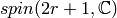
This is the Cartan type of . The last fundamental weight (1/2,
1/2, ... , 1/2) is the highest weight of the  dimensional spin
representation. All the other fundamental representations factor through the
homomorphism
dimensional spin
representation. All the other fundamental representations factor through the
homomorphism  and are representations of the
orthogonal group.
and are representations of the
orthogonal group.
The dominant weights consist of -tuples of integers or half-integers
 such that
  ,
and such that the differences
,
and such that the differences  .
.
sage: RootSystem("C3").ambient_space().simple_roots()
Finite family {1: (1, -1, 0), 2: (0, 1, -1), 3: (0, 0, 2)}
sage: RootSystem("C3").ambient_space().fundamental_weights()
Finite family {1: (1, 0, 0), 2: (1, 1, 0), 3: (1, 1, 1)}
sage: RootSystem("C3").ambient_space().rho()
(3, 2, 1)
This is the Cartan type of the symplectic group .
The dominant weights consist of -tuples of integers
such that
 .
.
sage: RootSystem("D4").ambient_space().simple_roots()
Finite family {1: (1, -1, 0, 0), 2: (0, 1, -1, 0), 3: (0, 0, 1, -1), 4: (0, 0, 1, 1)}
sage: RootSystem("D4").ambient_space().fundamental_weights()
Finite family {1: (1, 0, 0, 0), 2: (1, 1, 0, 0), 3: (1/2, 1/2, 1/2, -1/2), 4: (1/2, 1/2, 1/2, 1/2)}
sage: RootSystem("D4").ambient_space().rho()
(3, 2, 1, 0)
This is the Cartan type of . The last two fundamental weights are
the highest weights of the two  -dimensional spin
representations.
-dimensional spin
representations.
The dominant weights consist of -tuples of integers
such that
 .
.
We leave the reader to examine the exceptional types. You can use Sage to list the fundamental dominant weights and simple roots.
Let be a reductive complex analytic group. Let  be a
maximal torus,
be a
maximal torus,  be its group of analytic
characters. Then
be its group of analytic
characters. Then  for some
and
for some
and  .
.
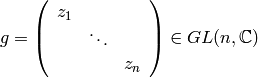
Example 1: Let  . Then is
the diagonal subgroup and
. Then is
the diagonal subgroup and 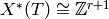 . If
. If 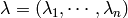 then
then  is identified with the rational
character
is identified with the rational
character
Example 2: Let  . Again is
the diagonal subgroup but now if
. Again is
the diagonal subgroup but now if
 then
then 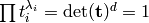 , so
, so 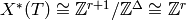 .
.
 are called weights.
 is any representation we may restrict
  to . Then the characters of that occur in this restriction are called the weights of . acts on its Lie algebra by conjugation (the adjoint representation). is
  .
.As we have mentioned, acts on its complexified Lie algebra
 by the adjoint representation. The zero weight space
 is just the Lie algebra of itself. The other
nonzero weights each appear with multiplicity one and form an interesting
configuration of vectors called the root system
is just the Lie algebra of itself. The other
nonzero weights each appear with multiplicity one and form an interesting
configuration of vectors called the root system  .
.
It is convenient to partition into two sets  and
and
 such that consists of all roots lying on one
side of a hyperplane. Often we arrange things so that is embedded in
such that consists of all roots lying on one
side of a hyperplane. Often we arrange things so that is embedded in
 in such a way that the positive weights correspond to upper
triangular matrices. Thus if
in such a way that the positive weights correspond to upper
triangular matrices. Thus if  is a positive root, its weight space
 is spanned by a vector
  , and the
exponential of this eigenspace in is a one-parameter subgroup of unipotent
matrices. It is always possible to arrange that this one-parameter subgroup
consists of upper triangular matrices.
, and the
exponential of this eigenspace in is a one-parameter subgroup of unipotent
matrices. It is always possible to arrange that this one-parameter subgroup
consists of upper triangular matrices.
If is a positive root that cannot be decomposed as a sum of other
positive roots, then is called a simple root. If is semisimple
of rank , then is the number of positive roots. Let
 be these.
Let be a complex analytic group. Let be a maximal torus, and let
 be its normalizer. Let
  be the Weyl group. It acts on
by conjugation; therefore it acts on the weight lattice and
its ambient space. The ambient space admits an inner product that is
invariant under this action. Let
be the Weyl group. It acts on
by conjugation; therefore it acts on the weight lattice and
its ambient space. The ambient space admits an inner product that is
invariant under this action. Let  denote this inner
product. If is a root let
denote this inner
product. If is a root let  denote the reflection in
the hyperplane of the ambient space that is perpendicular to .
If
denote the reflection in
the hyperplane of the ambient space that is perpendicular to .
If  is a simple root, then we use the notation
  to
denote .
to
denote .
Then  generate
  , which is a Coxeter group. This
means that it is generated by elements of order two and that
if
, which is a Coxeter group. This
means that it is generated by elements of order two and that
if  is the order of
  , then
is a presentation. An important function  is the length
function, where
is the length
function, where  is the length of the shortest decomposition of
  into a product of simple reflections.
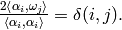
The coroots are certain linear functionals on the ambient space that also form a root system. Since the ambient space admits a $W$-invariant inner product, they may be identified with elements of the ambient space itself. Then they are proportional to the roots, though if the roots have different lengths, long roots correspond to short coroots and conversely. The coroot corresponding to the root $alpha$ is
$alpha^vee = frac{2alpha}{left<alpha,alpharight>}.$
The Dynkin Diagram is a graph whose vertices are in bijection
with the set simple roots. We connect the vertices corresponding
to roots that are not orthogonal. Usually two such vertices
make an angle of  , in which case we connect them
with a single bond. Occasionally they may make an angle
of
, in which case we connect them
with a single bond. Occasionally they may make an angle
of  in which case we connect them with a double
bond, or
in which case we connect them with a double
bond, or  in which case we connect them with a
triple bond. If the bond is single, the roots have the
same length with respect to the inner product on the ambient
space. In the case of a double or triple bond, the two simple
roots in questions have different length, and the bond is drawn
as an arrow from the long root to the short root. Only
the exceptional group has a triple bond.
in which case we connect them with a
triple bond. If the bond is single, the roots have the
same length with respect to the inner product on the ambient
space. In the case of a double or triple bond, the two simple
roots in questions have different length, and the bond is drawn
as an arrow from the long root to the short root. Only
the exceptional group has a triple bond.
There are various ways to get the Dynkin diagram:
sage: DynkinDiagram("D5")
        O 5
        |
        |
O---O---O---O
1   2   3   4
D5
sage: ct = CartanType("E6"); ct
['E', 6]
sage: ct.dynkin_diagram()
        O 2
        |
        |
O---O---O---O---O
1   3   4   5   6
E6
sage: B4=WeylCharacterRing("B4"); B4
The Weyl Character Ring of Type ['B', 4] with Integer Ring coefficients
sage: B4.dynkin_diagram()
O---O---O=>=O
1   2   3   4
B4
sage: RootSystem("G2").dynkin_diagram()
  3
O=<=O
1   2
G2
For the extended Dynkin diagram, we add one negative root
 . This is the root whose negative is the highest
weight in the adjoint representation. Sometimes this is called
the affine root. We make the Dynkin diagram as before by
measuring the angles between the roots. This extended Dynkin
diagram is useful for many purposes, such as finding maximal
subgroups and for describing the affine Weyl group.
. This is the root whose negative is the highest
weight in the adjoint representation. Sometimes this is called
the affine root. We make the Dynkin diagram as before by
measuring the angles between the roots. This extended Dynkin
diagram is useful for many purposes, such as finding maximal
subgroups and for describing the affine Weyl group.
The extended Dynkin diagram may be obtained as the Dynkin diagram of the corresponding untwisted affine type:
sage: ct = CartanType("E6"); ct
['E', 6]
sage: ct.affine()
['E', 6, 1]
sage: ct.affine() == CartanType(['E',6,1])
True
sage: ct.affine().dynkin_diagram()
        O 0
        |
        |
        O 2
        |
        |
O---O---O---O---O
1   3   4   5   6
E6~
The extended Dynkin diagram is also a method of the WeylCharacterRing:
sage: WeylCharacterRing("E7").extended_dynkin_diagram()
            O 2
            |
            |
O---O---O---O---O---O---O
0   1   3   4   5   6   7
E7~
There are certain weights  that:
that:
If is semisimple then these are uniquely determined, whereas if
is reductive but not semisimple we may choose them conveniently.
Let  be the sum of the fundamental dominant weights. If
is semisimple, then is half the sum of the positive
roots. In case is not semisimple, we have noted, the fundamental
weights are not completely determined by the inner product condition
given above. If we make a different choice, then is altered by
a vector that is orthogonal to all roots. This is a harmless change
for many purposes such as the Weyl character formula.
be the sum of the fundamental dominant weights. If
is semisimple, then is half the sum of the positive
roots. In case is not semisimple, we have noted, the fundamental
weights are not completely determined by the inner product condition
given above. If we make a different choice, then is altered by
a vector that is orthogonal to all roots. This is a harmless change
for many purposes such as the Weyl character formula.
In Sage, this issue arises only for Cartan type A. See SL versus GL.
Let be the group of rational characters. Then
.
are called weights. acts on , hence on and its ambient space by conjugation. has a fundamental domain
  for the Weyl group called the positive Weyl chamber. Weights in are called dominant. consists of all vectors such that
  for all positive roots . in
  and consider weights as lattice points.
 is a representation then restricting to , the module
  decomposes into a direct sum of weight eigenspaces
  with multiplicity
  for weight
  . with respect to the partial order. We have
  and
and  .
. gives a bijection between irreducible representations and weights in .
Assuming that is simply-connected (or more generally, reductive
with a simply-connected derived group) every dominant weight is the
highest weight of a unique irreducible representation  , and
, and
 gives a parametrization of the isomorphism classes
of irreducible representations of by the dominant weights.
gives a parametrization of the isomorphism classes
of irreducible representations of by the dominant weights.
The character of is the function  .
It is determined by its values on . If
.
It is determined by its values on . If  and
and  ,
let us write
,
let us write  for the value of on
  . Then
the character:
. Then
the character:
 .
.
Sometimes this is written
 .
.
The meaning of  is subject to interpretation, but we may regard it as
the image of the additive group in its group algebra. The character
is then regarded as an element of this ring, the group algebra of .
is subject to interpretation, but we may regard it as
the image of the additive group in its group algebra. The character
is then regarded as an element of this ring, the group algebra of .
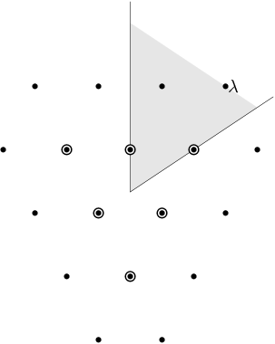
In this example,  . We have drawn the
weights of an irreducible representation with highest weight .
The shaded region is . is a dominant
weight, and the labeled vertices are the weights with positive multiplicity in
. We have drawn the
weights of an irreducible representation with highest weight .
The shaded region is . is a dominant
weight, and the labeled vertices are the weights with positive multiplicity in
 . The weights weights on the outside have
  ,
while the six interior weights (with double circles) have
,
while the six interior weights (with double circles) have  .
.
The considerations of this section are particular to type A. We review
the relationship between characters of and
symmetric function theory.
A partition is a sequence of descending nonnegative
integers:

We do not distinguish between two partitions if they differ only by some
trailing zeros, so  . If
. If  is the last integer such that
 then we say that is the length of . If
 then we say that is a partition of
and write
then we say that is a partition of
and write  .
.
A partition of length  is therefore a dominant weight of type ['A',r].
Not every dominant weight is a partition, since the coefficients in a dominant
weight could be negative. Let us say that an element
is therefore a dominant weight of type ['A',r].
Not every dominant weight is a partition, since the coefficients in a dominant
weight could be negative. Let us say that an element  of the ['A',r] root lattice is effective if the
  . Thus an effective
dominant weight of ['A',r] is a partition of length
. Thus an effective
dominant weight of ['A',r] is a partition of length  , where
  .
.
Let be a dominant weight, and let  be the character
of with highest weight . If is any integer
we may consider the weight
be the character
of with highest weight . If is any integer
we may consider the weight  obtained by adding to each entry. Then
  .
Clearly by choosing large enough, we may make
.
Clearly by choosing large enough, we may make  effective.
So the characters of irreducible representations of
do not all correspond to partitions, but the characters indexed by
partitions (effective dominant weights) are enough that we can
write any character  where is a
partition. If we take
where is a
partition. If we take  we could also arrange that
the last entry in is zero.
we could also arrange that
the last entry in is zero.
If is an effective dominant weight, then every weight that
appears in is effective. (Indeed, it lies in the convex
hull of  where runs through the Weyl group
  .)
This means that if
.)
This means that if
then  is a polynomial in the eigenvalues of .
This is the Schur polynomial
is a polynomial in the eigenvalues of .
This is the Schur polynomial  .
.