Let $W$ be the symmetric group $S_n$. It is a Coxeter group with generators $s_1, \cdots, s_{n - 1}$. Let $w \in S_n$ and let $\mathfrak{w}= (i_1, \cdots, i_l)$ be a reduced word for $w$, so that $w = s_{i_1} \cdots s_{i_l}$ is a decomposition of shortest possible length into simple reflections. Edelman-Greene insertion is a variant of RSK that is adapted to reduced words. It is connected with the theory of Stanley symmetric functions, which can be used to count reduced words, and Morse-Schilling crystals whose characters are Stanley symmetric functions. Edelman-Green insertion resembles dual RSK

By a tableau we will always mean a semistandard Young tableau $T$ (in English notation). The tableau is called strict if the rows, as well as the columns are strictly increasing. If the tableau is a row, let

\[ \text{word} (T) = (i_1, \cdots, i_s), \hspace{2em} T = \begin{array} {|l|l|l|l|} \hline i_1 & i_2 & \cdots & i_s\\ \hline \end{array} . \]

(2.1)

More generally, if $T_1, \cdots, T_r$ are the rows of $T$, let $\text{word} (T)$ be obtained by concatenating $\text{word} (T_r), \cdots, \text{word} (T_1)$. Thus $\text{word} (T)$ is the reading word of $T$, reading row by row, starting with the bottom row and reading each row from left to right. Then $T$ is called reduced if $\text{word} (T)$ is a reduced word for $w$ where $w = s_{i_1} \cdots s_{i_r}$. In this case we will also write $w (T) = w$. Clearly a reduced tableau is strict.

We call the tableau $T$ standard if its entries are $1, 2, 3, \cdots, r$, each appearing exactly once, where $r$ is the size of $T$. Clearly a standard tableau is strict.

Edelman-Greene insertion (EG) is a variant of RSK. Let $T$ be a tableau and $k$ an integer. We assume that $T$ is reduced. Let $\text{word} (T) = (i_1, \cdots, i_s)$ and assume that $T$ is a reduced word for $w = s_{i_1} \cdots s_{i_s}$. Let $k$ be a right ascent for $w$, so that the length $l (ws_k) = s + 1$. We will describe a new tableau $T \leftarrow k$ obtained by the following insertion algorithm. First suppose that $T$ is the row (2.1). If $k > i_s$ then we define $T \leftarrow k$ to be \[ \begin{array} {|l|l|l|l|l|} \hline i_1 & i_2 & \cdots & i_s & k\\ \hline \end{array} . \] Let us call this type of insertion Case 1.

On the other hand if $k \leqslant i_s$ then our assumption that $k$ is an ascent for $w$ implies that $k < i_s$. Let $u$ be the smallest positive integer such that $k < i_u$. Let $k' = i_u$. There are two cases. If $u = 1$ or if $u > 1$ and $i_{u - 1} < k$ then $T \leftarrow k$ is

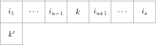
Let us call this type of insertion Case 2. This coincides with RSK insertion.

On the other hand if $u > 1$ and $i_{u - 1} = k$ then our assumption that $k$ is an ascent for $w$ implies that $i_u = k + 1$, since otherwise $s_k$ commutes with $s_{i_u} \cdots s_{i_s}$ and therefore $ws_k = s_{i_1} \cdots s_{i_{u - 2}} s_{i_u} \cdots s_{i_s}$ has length $< l (w)$. In this case $T \leftarrow k$ is

In this Case 3 insertion we have \[ i_{u - 1} = k, i_u = k' = k + 1. \] This differs from RSK insertion in that the top row is unchanged.

In both situations we will also use the notation $k' \leftarrow T'$ for the tableau $T \leftarrow k$. In these last two cases we say that $k'$ is bumped on insertion. We will also denote by $\beta (T \leftarrow k) = u$ the location of the bumped entry.

Now that we have defined EG insertion in the case the tableau is a row, let us consider the general case. Let $T_1, \cdots, T_r$ be the rows of the reduced tableau $T$. We will replace several of these, $T_1, \cdots, T_q$ by new rows $T_1', \cdots, T_q'$ and $T \leftarrow k$ will be the tableau with rows $T_1', \cdots, T_q', T_{q + 1}, \cdots, T_r$.

If $T_1 \leftarrow k$ is a row $T_1'$, the algorithm terminates. That is, $q = 1$ and $T_1' = T \leftarrow k$. We have simply added an entry $k$ at the end of the first row.

Otherwise, suppose that $k_1$ is bumped, so $(T_1 \leftarrow k) = (k_1 \leftarrow T_1')$ for a row $T_1'$. Either one entry $i_u$ in $T_1$ has been replaced by a smaller entry $k$, or $T_1' = T_1$. Now let us insert $k_1$ into $T_2$. If $T_2 \leftarrow k_1$ is a tableau $T_2'$, then $q = 2$ and the algorithm terminates. We have added $k_1$ at the end of the second row. On the other hand if $k_2$ is bumped, so that $(T_2 \leftarrow k_1) = (k_2 \leftarrow T_2')$ then we continue inserting $k_2$ into $T_3$, etc.

Lemma 2.1: $T_1', \cdots, T_q', T_{q + 1}, \cdots, T_r$ are the rows of a tableau $T \leftarrow k$.

Proof. (Click to Expand/Collapse)

Let $\beta_i = \beta (T_i, k_{i - 1})$ be the sequence of bump locations. (Here we denote $k_0 = k$.) Each Case 2 insertion in a row $T_i$ with $i > 1$ decreases the $\beta_i$-th entry of $T_i$ to $k_{i - 1}$, and what must be checked that the value above it in $T_{i - 1}'$ is less than $k_{i - 1}$. Let $u_1, u_2, \cdots$ be the entries in $T_{i - 1}$ and let $v_1, v_2, \cdots$ be the entries in $T_i$. It follows from the definition of $T_i \leftarrow k_{i - 1}$ that $\beta_i \leqslant \beta_{i - 1}$ since $k_{i - 1} = u_{\beta_i}$ cannot be inserted to the right of $v_{\beta_{i - 1}}$ which is $> u_{\beta_{i - 1}}$. There are two cases to consider. If $\beta_i < \beta_{i - 1}$ then $u_{\beta_i} < u_{\beta_{i - 1}} = k_{i - 1}$ since $T$ is strict. Therefore suppose that $\beta_i = \beta_{i - 1}$. If the insertion in $T_{i - 1}$ is Case 2 then the $\beta_{i - 1}$ entry has already been decreased from $k_{i - 1}$ in $T'_{i - 1}$. Thus let us assume that the insertion in $T_{i - 1}$ is Case 3. Then $u_{\beta_i} = k_{i - 1}$, $u_{\beta_i - 1} = k_{i - 1} - 1$ and since $T$ is column strict $v_{\beta_i - 1} \geqslant k_{i - 1}$. We also have $v_{\beta_i - 1} \leqslant k_{i - 1}$ since otherwise $\beta_i$ would be $< \beta_{i - 1}$. So $v_{\beta_i - 1} = k_{i - 1}$. Because we are assuming that the insertion in row $T_i$ is Case 3 it follows that $T_i'$ has two consecutive entries $v_{\beta_i - 1}$ and $v_{\beta_i}$ that are both equal to $k_i - 1$. This is a contradiction since $T_i'$ is strict.

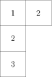
If $T$ is a tableau, we recall that the reading word $\omega (T)$ of $T$ is obtained by reading the rows from left to right, starting with the bottom row and moving upwards. If $\omega (T) = (i_1, \cdots, i_k)$ let $w (T) = s_{i_1} \cdots s_{i_k}$. For example, suppose that $T$ is

Then $\omega (T) = (3, 1, 2)$ and $w (T) = s_3 s_1 s_2$. The tableau $T \leftarrow 1$ is

We note that $w (T \leftarrow 1) = s_3 s_2 s_1 s_2 = s_3 s_1 s_2 s_1 = w (T) \, s_1$. This is a special case of the following Lemma.

Lemma 2.2: Suppose that $T$ is a reduced tableau and that $k$ is a right ascent of $w (T)$. Then $w (T \leftarrow k) = w (T) \hspace{0.25em} s_k$.

Proof. (Click to Expand/Collapse)

We reduce easily to the case where $T$ is a row. If the insertion is Case 1 the assertion is obvious. For Case 2 and Case 3 insertions, $T \leftarrow k$ has two rows and the second row is a single block $ \begin{array} {|l|} \hline k'\\ \hline \end{array} $. For Case 2 insertions, $s_{i_u} = s_{k'}$ commutes with $s_{i_1} \cdots s_{i_{u - 1}}$ while $s_k$ commutes with $s_{i_{u + 1}} \cdots s_{i_s}$, and so \[ w (T) s_k = s_{i_1} \cdots s_{i_{u - 1}} s_{k'} s_{i_{u + 1}} \cdots s_{i_s} s_k = s_{k'} s_{i_1} \cdots s_{i_{u - 1}} s_k s_{i_{u + 1}} \cdots s_{i_s} = s_{k'} w (T) . \] For Case 3 we have \[ w (T) s_k = s_{i_1} \cdots s_{i_{u - 2}} s_k s_{k + 1} s_{i_{u + 1}} \cdots s_{i_s} s_k = s_{i_1} \cdots s_{i_{u - 2}} s_k s_{k + 1} s_k s_{i_{u + 1}} \cdots s_{i_s} . \] Now using the braid relation $s_k s_{k + 1} s_k = s_{k'} s_k s_{k + 1}$ with $k' = k + 1$ \[ s_{i_1} \cdots s_{i_{u - 2}} s_{k'} s_k s_{k + 1} s_{i_{u + 1}} \cdots s_{i_s} = s_{k'} s_{i_1} \cdots s_{i_{u - 2}} s_k s_{k + 1} s_{i_{u + 1}} \cdots s_{i_s} = s_{k'} w (T) . \]

Now let $\mathfrak{w} = (i_1, \cdots, i_m)$ be a reduced word for $w \in S_{r + 1}$. We will define two tableaux $P ( \mathfrak{w})$ and $Q ( \mathfrak{w})$ of the same shape $\lambda$, a partition of $m$. The tableau $P ( \mathfrak{w})$ will be reduced, and the tableau $Q ( \mathfrak{w})$ will be standard. We build up $P ( \mathfrak{w})$ by successively inserting $i_1, \cdots, i_m$ into the empty tableau $\varnothing$; that is, \[ P ( \mathfrak{w}) = \varnothing \leftarrow i_1 \leftarrow i_2 \leftarrow \ldots \leftarrow i_m . \] By Lemma 2.2 we have $w = w (P ( \mathfrak{w}))$. The tableaux $Q ( \mathfrak{w})$ is the recording tableau, as in the usual RSK algorithm: the entries are the locations of the successive insertions.

For example, suppose that $\mathfrak{w} = (2, 3, 2, 1, 2)$. Then

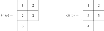
Theorem 2.1: (Edelman-Greene) Let $w$ be a permutation. Then the map $\mathfrak{w} \mapsto (P ( \mathfrak{w}), Q ( \mathfrak{w}))$ is a bijection between reduced words for $w$ and pairs $(P, Q)$ of tableaux of the same shape such $P$ is reduced and $Q$ standard, with $w = w (P)$.

Note that $\text{word} (P ( \mathfrak{w}))$ is different from $\mathfrak{w}$, though they are both reduced words for the $w$.

Proof. (Click to Expand/Collapse)

To see that this map is a bijection, we observe that there is an inverse construction. Let $P$ and $Q$ be given. It is assumed that they are tableau with the same shape $\lambda$, a partition of $m$, with $P$ reduced and $Q$ standard; and $w = w (P)$. The location of $m$ in $Q$ is an extremal location for the shape $\lambda$. Let $\lambda_{m - 1}$ be the shape obtained by removing this location from the shape $\lambda$, and let $Q_{m - 1}$ be the shape obtained by removing this location from $Q$.

By running the EG construction in reverse, we may find a tableau $P_{m - 1}$ of shape $\lambda_{m - 1}$ and a value $i_m$ such that $P = P_{m - 1} \leftarrow i_m$. We repeat the process with $P$ and $Q$ replaced by $P_{m - 1}$ and $Q_{m - 1}$ to reconstruct the unique sequence $\mathfrak{w} = (i_1, \cdots, i_m)$ such \[ (P ( \mathfrak{w}), Q ( \mathfrak{w})) = (P, Q) . \]

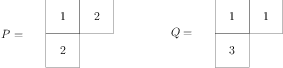
To illustrate this, in the above example, $m = 5$ and $\lambda_4$ is the partition $(2, 1, 1)$. Since the insertions are to terminate in the second row \ at the location of $5$ in $Q$. Thus the second row of $P_4$ should be $ \begin{array} {|l|} \hline 2\\ \hline \end{array} $ and the top row should be $ \begin{array} {|l|l|} \hline 1 & 3\\ \hline \end{array} $ since $ \begin{array} {|l|l|} \hline 1 & 3\\ \hline \end{array} \leftarrow 2$ equals $3 \leftarrow \begin{array} {|l|l|} \hline 1 & 2\\ \hline \end{array} $. We find that

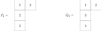
Theorem 2.2: (Stanley) Let $n$ be given. The number of reduced words of the long element $w_0 \in S_n$ equals the number of standard tableaux of shape $\rho = (n - 1, n - 2, \cdots, 1)$.

Proof. (Click to Expand/Collapse)

In the bijection of Theorem 2.1, there is only one possible choice for $P$. Indeed, there can be only one reduced tableau for $w_0$ because such a tableau must be strict and of size $\frac{1}{2} n (n - 1)$, and there is only one such tableau in the alphabet $\{1, 2, 3, \cdots, n\}$. Its shape is $\rho$. Hence the number of reduced words is the number of standard tableaux $Q$ with this shape.

There is a variant of Edelman-Green that is analogous to dual RSK for (0,1) matrices. This leads to the Morse-Schilling crystals, whose characters are the Stanley symmetric functions.

This may be expressed in the following manner. Let $k$ be a positive integer. Let $w \in S_n$ be called increasing if it has a reduced word $(i_1, i_2, \cdots)$ such that $i_1 < i_2 < \cdots$. If it has such a reduced word, the word in unique.

An increasing factorization of length $k$ is a decomposition $w = w_1 w_2 \cdots w_k$ where $w_i$ is increasing, and $l (w) = \sum l (w_i)$. As Morse and Schilling observed, these may be given the structure of a $\operatorname{GL} (k)$ crystal. The weight of a decomposition, regarded as a crystal element is $(\lambda_1, \lambda_2, \cdots)$ where $\lambda_i = l (w_i)$. We will change the setup a little by considering increasing decompositions (instead of decreasing ones), and the crystal we describe will have its character the Stanley symmetric function, $f_{w^{- 1}}$. Our reason for making these changes is to be compatible with our RSK conventions.

We will explain later how the crystal structure arises, but first let us give some examples.

For the first let $w = s_1 s_2$. Take $k = 3$. The crystal graph of the Morse-Schilling crystal is

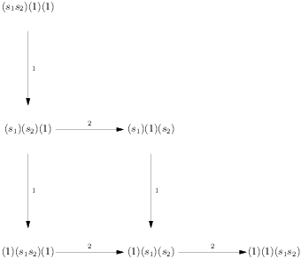
This resembles the crystal graph of the $\operatorname{GL} (3)$ crystal of rows $\mathcal{B}_{(2)}$.

Next suppose that $w = s_2 s_1$ and $k = 3$. Then there are only 3 factorizations, $(s_2) (s_1) (1)$, $(s_2) (1) (s_1)$ and $(1) (s_2) (s_1)$.

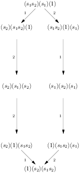
For a final example, let $w = s_1 s_2 s_1$ be the long element of $S_3$ and let $k = 3$. Then the crystal graph of the Morse-Schilling crystal looks like this:

This resembles the crystal graph of the $\operatorname{GL} (3)$ crystal $\mathcal{B}_{(2, 1)}$. In these three examples, the crystal is connected, but in other examples, it is not.

Theorem 2.3: Let $w \in S_n$. There is a bijection increasing factorizations of $w$ between pairs $(P, Q)$ of tableaux, in which $Q$ is a semistandard tableau in the alphabet $[k]$, and $P$ is a tableau of the same shape as $Q$ in the alphabet $[n - 1]$ such that the reading word of $P$ is a reduced word for $w$.

Before giving the proof we describe the bijection. Given an increasing factorization $w = w_1 \cdots w_k$, we construct a two-rowed array with the columns $A$ in lexicographical order. There will be no repeated columns, so this is the two-rowed array of a (0,1) matrix.

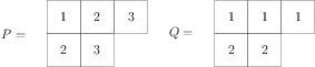
The increasing element $w_i$ has a unique reduced word $(m_{i, 1}, m_{i, 2}, \cdots)$ with $m_{i, 1} < m_{i, 2} < \cdots$. We put the $m_{i, j}$ as the second row entries with $i$ in the first row. Thus for the decomposition $(s_1 s_2) (1) (s_1)$ of $w = s_1 s_2 s_1$, the two-rowed matrix is \[ \left( \begin{array} {ccc} 1 & 1 & 3\\ 1 & 2 & 1 \end{array} \right) . \] Now we construct the pair $(P, Q)$ just as in the usual RSK algorithm by successively inserting the bottom row entries into the empty tableau, putting the top row entries into the recording tableau. We use EG insertion instead of RSK. Thus in this example, we have

Proof. (Click to Expand/Collapse)

Most of the things that need to be checked are the same as in Theorem 2.1, except to recover the two-rowed array from $(P, Q)$ we we need to know how to determine the landing locations from the recording tableau. (If that is known, we may run the algorithm in reverse as in Theorem 2.1.) This detail is similar to the corresponding point in Theorem 2.3. Let $t$ be the highest entry in $Q$. No two entries equal to $t$ can occur in the same column, since $Q$ is semistandard. The one farthest to the right is the landing location. This is a consequence of the fact that the bottom row entries of the two-rowed array corresponding to $t$ are increasing, and have been inserted in order, and a bit of thought will show that their landing locations are ordered from left to right.

There are two approaches to the problem of giving a crystal structure the set of increasing factorizations of $w$.

We may define the Kashiwara operators on the pairs $(P, Q)$ in Theorem 2.3 by letting them act as the usual tableau operators on $Q$, while fixing $P$. By transportation of structure, there is then an operator on increasing factorizations of $w$.
Schilling and Morse give a direct definition on reduced words, and verify that the Stembridge axioms are satisfied. Then they check compatibility with Edelman-Greene insertion.

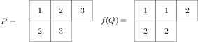
Here is an example. Consider the $\operatorname{GL} (2)$ Morse-Schilling crystal whose highest weight vector is the word $(s_1 s_2 s_3) (s_1 s_2)$, which we abbreviate as $(123) (12)$. We make the two-rowed array: \[ \left( \begin{array} {ccccc} 1 & 1 & 1 & 2 & 2\\ 1 & 2 & 3 & 1 & 2 \end{array} \right) . \] Edelman-Greene insertion produces the following pair of tableaux. The second one is $Q$.

Applying $f = f_1$ to $Q$, we need to apply reverse Edelman-Greene to the tableaux:

The landing location of the last insertion is at the rightmost $2$ in $f (Q)$, and so the last insertion is $3$. We thus begin to work backwards and reconstruct the two-rowed array: \[ \begin{array} {|l|} \hline \begin{array} {ll} 1 & 2\\ 2 & 3 \end{array} \\ \hline \end{array} \hspace{2em} \begin{array} {|l|} \hline \begin{array} {ll} 1 & 1\\ 2 & 2 \end{array} \\ \hline \end{array} \hspace{2em} \left( \begin{array} {ccccc} 1 & 1 & 2 & 2 & 2\\ ? & ? & ? & ? & 3 \end{array} \right) \] \[ \begin{array} {|l|} \hline \begin{array} {ll} 1 & 3\\ 2 & \end{array} \\ \hline \end{array} \hspace{2em} \begin{array} {|l|} \hline \begin{array} {ll} 1 & 1\\ 2 & \end{array} \\ \hline \end{array} \hspace{2em} \left( \begin{array} {ccccc} 1 & 1 & 2 & 2 & 2\\ ? & ? & ? & 2 & 3 \end{array} \right) \] \[ \begin{array} {|l|} \hline \begin{array} {ll} 2 & 3 \end{array} \\ \hline \end{array} \hspace{2em} \begin{array} {|l|} \hline \begin{array} {ll} 1 & 1 \end{array} \\ \hline \end{array} \hspace{2em} \left( \begin{array} {ccccc} 1 & 1 & 2 & 2 & 2\\ ? & ? & 1 & 2 & 3 \end{array} \right) \] \[ \left( \begin{array} {ccccc} 1 & 1 & 2 & 2 & 2\\ 2 & 3 & 1 & 2 & 3 \end{array} \right) \] Finally we deduce that \[ f ((123) (12)) = (23) (123) . \] As a sanity check let us show that $s_1 s_2 s_3 s_1 s_2 = s_2 s_3 s_1 s_2 s_3$ in $S_4$ using the braid relations: \[ s_1 s_2 s_3 s_1 s_2 = s_1 s_2 s_1 s_3 s_2 = s_2 s_1 s_2 s_3 s_2 = s_2 s_1 s_3 s_2 s_3 = s_2 s_3 s_1 s_2 s_3 . \]

Now let us recall how Morse and Schilling describe the operators $f_i$. We recall that they word with decreasing words instead of increasing ones, but it is trivial to translate their algorithm to this context.

The operators $e_i$ and $f_i$ acts only on a pair $w_i$, $w_{i + 1}$ of adjacent words in an increasing factorization. The content $\operatorname{cont} (w)$ of an increasing word $w$ is the set of letters in its reduced word. Roughly, $e_i$ will remove one element $b$ from $\operatorname{cont} (w_{i + 1})$ and add a single element $b - t$ from $\operatorname{cont} (w_i)$. In other words, $e_i (w_i w_{i + 1}) = \widetilde{w_i} \tilde{w}_{i + 1}$ where $\operatorname{cont} ( \tilde{w}_{i + 1}) = \operatorname{cont} (w_{i + 1}) -\{b\}$ and $\operatorname{cont} ( \widetilde{w_i}) = \operatorname{cont} (w_i) \cup \{b - t\}$ where $b$ and $b - t$ remain to be described. It will be the case that $w_i w_{i + 1} = \widetilde{w_i} \tilde{w}_{i + 1}$. Similarly $f_i$ removes one element $a$ from $\operatorname{cont} (w_{i + 1})$ and adjoins an element $a + s$ to $\operatorname{cont} (w_i)$.

To describe the algorithm precisely, they begin by "bracketing'' or pairing up elements of the content of $w_i$ and $w_{i + 1}$. They start with the largest letter $x$ in $\operatorname{cont} (w_{i + 1})$ and pair it with the smallest $y > x$ in $\operatorname{cont} (w_i)$. If there is no such letter, then $x$ is left unpaired. The process repeats on the unpaired elements until no pairings are found. Thus in the pairing $(123) (12)$ the $x = 2$ in $\operatorname{cont} (w_2) =\{1, 2\}$ is paired with $3$ in $\operatorname{cont} (w_1) =\{1, 2, 3\}$. Removing these from consideration, the largest unpaired element in $\operatorname{cont} (w_2)$ is 1, which is paired with $2$ in $\operatorname{cont} (w_1)$. We indicate this by bracketing the paired elements. \[ (1 [2] [3]) ([1] [2]) \]

If every element of $\operatorname{cont} (w_i)$ is bracketed, then $f_i (w_i w_{i + 1}) = 0$. We assume that this is not the case. Then let $a$ be the largest unbracketed element of $w_i$, and let $a + s$ be the smallest integer $\geqslant 0$ such that $a + s + 1 \notin \operatorname{cont} (w_i)$.

In the example, $a = 1$ and $a + s = 3$. So $f_1$ removes $a$ from $\operatorname{cont} (w_1)$ and adds $3$ to $\operatorname{cont} (w_2)$. Thus \[ f_1 ((123) (12)) = (23) (123) . \]

[To be continued!]