If  is a Lie group and
  is a subgroup, one often needs to
know how representations of restrict to . Irreducibles
usually do not restrict to irreducibles. In some cases the restriction is
regular and predictable, in other cases it is chaotic. The description of how
irreducibles decompose into irreducibles is called a branching rule.
is a subgroup, one often needs to
know how representations of restrict to . Irreducibles
usually do not restrict to irreducibles. In some cases the restriction is
regular and predictable, in other cases it is chaotic. The description of how
irreducibles decompose into irreducibles is called a branching rule.
References for this topic:
Sage has enough built in branching rules to handle all cases where
is a classical group, that is, type A, B, C or D. It also has many built in
cases where is an exceptional group.
Clearly it is sufficient to consider the case where is a maximal
subgroup of , since if this is known then one may branch down
successively through a series of subgroups, each maximal in its
predecessors. A problem is therefore to understand the maximal subgroups in a
Lie group, and to give branching rules for each.
For convenience Sage includes some branching rules to non-maximal subgroups, but strictly speaking these are not necessary. The goal is to give a sufficient set of built-in branching rules for all maximal subgroups, and this is accomplished for classical groups (types A, B, C or D) at least up to rank 8, and for many maximal subgroups of exceptional groups.
A Levi subgroup may or may not be maximal. They are easily classified. If one
starts with a Dynkin diagram for and removes a single node, one
obtains a smaller Dynkin diagram, which is the Dynkin diagram of a smaller
subgroup .
For example, here is the A3 Dynkin diagram:
sage: A3=WeylCharacterRing("A3")
sage: A3.dynkin_diagram()
O---O---O
1   2   3
A3
We see that we may remove the node 3 and obtain A2,
or the node 2 and obtain A1xA1. These correspond to the
Levi subgroups  and
and 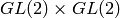 of
of
 . Let us construct the irreducible representations
of and branch them down to these down to
and :
. Let us construct the irreducible representations
of and branch them down to these down to
and :
sage: A3=WeylCharacterRing("A3")
sage: reps = [A3(v) for v in A3.fundamental_weights()]; reps
[A3(1,0,0,0), A3(1,1,0,0), A3(1,1,1,0)]
sage: A2=WeylCharacterRing("A2")
sage: A1xA1=WeylCharacterRing("A1xA1")
sage: [pi.branch(A2,rule="levi") for pi in reps]
[A2(0,0,0) + A2(1,0,0), A2(1,0,0) + A2(1,1,0), A2(1,1,0) + A2(1,1,1)]
sage: [pi.branch(A1xA1,rule="levi") for pi in reps]
[A1xA1(0,0,1,0) + A1xA1(1,0,0,0),
 A1xA1(0,0,1,1) + A1xA1(1,0,1,0) + A1xA1(1,1,0,0),
 A1xA1(1,0,1,1) + A1xA1(1,1,1,0)]
Let us redo this calculation in coroot notation. As we have
explained, coroot notation does not distinguish between representations
of that have the same restriction to  , so in
effect we are now working with the groups and its
Levi subgroups
, so in
effect we are now working with the groups and its
Levi subgroups  and
and  :
:
sage: A3=WeylCharacterRing("A3",style="coroots")
sage: reps = [A3(v) for v in A3.fundamental_weights()]; reps
[A3(1,0,0), A3(0,1,0), A3(0,0,1)]
sage: A2=WeylCharacterRing("A2",style="coroots")
sage: A1xA1=WeylCharacterRing("A1xA1",style="coroots")
sage: [pi.branch(A2,rule="levi") for pi in reps]
[A2(0,0) + A2(1,0), A2(0,1) + A2(1,0), A2(0,0) + A2(0,1)]
sage: [pi.branch(A1xA1,rule="levi") for pi in reps]
[A1xA1(0,1) + A1xA1(1,0), 2*A1xA1(0,0) + A1xA1(1,1), A1xA1(0,1) + A1xA1(1,0)]
Now we may observe a distinction difference in branching from
 and with
  . Consider the middle representation, which is the six
dimensional exterior square. In the coroot notation, the
restriction contained two copies of the trivial
representation, 2*A1xA1(0,0). The other way, we had instead
three distinct representations in the restriction, namely
A1xA1(1,1,0,0) and A1xA1(0,0,1,1), that is,
. Consider the middle representation, which is the six
dimensional exterior square. In the coroot notation, the
restriction contained two copies of the trivial
representation, 2*A1xA1(0,0). The other way, we had instead
three distinct representations in the restriction, namely
A1xA1(1,1,0,0) and A1xA1(0,0,1,1), that is,  and
and  .
.
The Levi subgroup A1xA1 is actually not maximal. Indeed, we may factor the embedding:

Therfore there are branching rules A3 -> C2 and C2 -> A2, and we could accomplish the branching in two steps, thus:
sage: A3 = WeylCharacterRing("A3",style="coroots")
sage: C2 = WeylCharacterRing("C2",style="coroots")
sage: B2 = WeylCharacterRing("B2",style="coroots")
sage: D2 = WeylCharacterRing("D2",style="coroots")
sage: A1xA1=WeylCharacterRing("A1xA1",style="coroots")
sage: reps = [A3(fw) for fw in A3.fundamental_weights()]
sage: [pi.branch(C2,rule="symmetric").branch(B2,rule="isomorphic").\
....:     branch(D2,rule="extended").branch(A1xA1,rule="isomorphic") for pi in reps]
[A1xA1(0,1) + A1xA1(1,0), 2*A1xA1(0,0) + A1xA1(1,1), A1xA1(0,1) + A1xA1(1,0)]
As you can see, we’ve redone the branching rather circuitously this way, making use of the branching rules A3->C2 and B2->D2, and two accidental isomorphisms C2=B2 and D2=A1xA1. It is much easier to go in one step using rule="levi", but reassuring that we get the same answer!
It is also true that if we remove one node from the extended Dynkin diagram that we obtain the Dynkin diagram of a subgroup. For example:
sage: G2=WeylCharacterRing("G2",style="coroots")
sage: G2.extended_dynkin_diagram()
  3
O=<=O---O
1   2   0
G2~
Observe that by removing the 1 node that we obtain an A2
Dynkin diagram. Therefore the exceptional group G2 contains
a copy of . We branch the two representations of G2
corresponding to the fundamental weights to this copy of A2:
sage: G2=WeylCharacterRing("G2",style="coroots")
sage: A2=WeylCharacterRing("A2",style="coroots")
sage: [G2(f).degree() for f in G2.fundamental_weights()]
[7, 14]
sage: [G2(f).branch(A2,rule="extended") for f in G2.fundamental_weights()]
[A2(0,0) + A2(0,1) + A2(1,0), A2(0,1) + A2(1,0) + A2(1,1)]
The two representations of G2, of degrees 7 and 14 respectively are the action on the octonions of trace zero and the adjoint representation.
For embeddings of this type, the rank of the subgroup is
the same as the rank of . This is in contrast with
embeddings of Levi type, where has rank one less than .
If  then has a subgroup
 . This lifts to an embedding
of the universal covering groups
. This lifts to an embedding
of the universal covering groups

Sometimes this embedding is of extended type, and sometimes
it is not. It is of extended type unless  and
and  are both
odd. If it is of extended type then you may use
rule="extended". In any case you may use rule="orthogonal_sum".
The name refer to the origin of the embedding
are both
odd. If it is of extended type then you may use
rule="extended". In any case you may use rule="orthogonal_sum".
The name refer to the origin of the embedding  from the decomposition of the underlying quadratic space
as a direct sum of two orthogonal subspaces.
from the decomposition of the underlying quadratic space
as a direct sum of two orthogonal subspaces.
There are four cases depending on the parity of and
. For example, if  and
and  we
have an embedding :
we
have an embedding :
['D',k] x ['D',l] --> ['D',k+l]
This is of extended type. Thus consider the embedding D4xD3 -> D7. Here is the extended Dynkin diagram:
  0 O           O 7
    |           |
    |           |
O---O---O---O---O---O
1   2   3   4   5   6
Removing the 4 vertex results in a disconnected Dynkin diagram:
  0 O           O 7
    |           |
    |           |
O---O---O       O---O
1   2   3       5   6
This is D4xD3. Therefore use the “extended” branching rule:
sage: D7=WeylCharacterRing("D7",style="coroots")
sage: D4xD3=WeylCharacterRing("D4xD3",style="coroots")
sage: spin = D7(D7.fundamental_weights()[7]); spin
D7(0,0,0,0,0,0,1)
sage: spin.branch(D4xD3,rule="extended")
D4xD3(0,0,1,0,0,1,0) + D4xD3(0,0,0,1,0,0,1)
Similarly we have embeddings
['D',k] x ['B',l] --> ['B',k+l].
These are also of extended type. For example consider the embedding of D3xB2->B5. Here is the B5 extended Dynkin diagram:
    O 0
    |
    |
O---O---O---O=>=O
1   2   3   4   5
Removing the 3 node gives:
    O 0
    |
O---O       O=>=O
1   2       4   5
and this is the Dynkin diagram or D3xB2. For such branchings we again use rule="extended".
Finally, there is an embedding
['B',k] x ['B',l] --> ['D',k+l+1]
This is not of extended type, so you may not use rule="extended".
If admits an outer automorphism (usually of order two) then
we may try to find the branching rule to the fixed subgroup .
It can be arranged that this automorphism maps the maximal torus
 to itself and that a maximal torus
  of is contained
in .
of is contained
in .
Suppose that the Dynkin diagram of admits an automorphism. Then
itself admits an outer automorphism. The Dynkin diagram of the
group of invariants may be obtained by “folding” the Dynkin
diagram of along the automorphism. The exception is the
branching rule  .
.
Here are the branching rules that can be obtained using rule="symmetric".
|
|
Cartan Types |
|---|---|---|
 |
 |
[‘A’,2r-1] => [‘C’,r] |
 |
 |
[‘A’,2r] => [‘B’,r] |
|
 |
[‘A’,2r-1] => [‘D’,r] |
|
 |
[‘D’,r] => [‘B’,r-1] |
 |
 |
[‘E’,6] => [‘F’,4] |
If  and
and  are Lie groups, and we have representations
 and
and  then the tensor
product is a representation of
then the tensor
product is a representation of  . It has its image
in
. It has its image
in  but sometimes this is conjugate to a subgroup of
 or
or  . In particular we have the following cases.
| Group | Subgroup | Cartan Types |
|---|---|---|
 |
 |
['A', rs-1] => ['A',r-1] x ['A',s-1] |
 |
 |
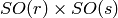
['B',2rs+r+s] => ['B',r] x ['B',s] |
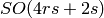 |
 |
['D',2rs+s] => ['B',r] x ['D',s] |
 |
 |
['D',2rs] => ['D',r] x ['D',s] |
|
 |
['D',2rs] => ['C',r] x ['C',s] |
 |
 |
['C',2rs+s] => ['B',r] x ['C',s] |
 |
 |
['C',2rs] => ['C',r] x ['D',s] |
These branching rules are obtained using rule="tensor".
The k-th symmetric and exterior power homomorphisms
map  and
and  . The
corresponding branching rules are not implemented but a special
case is. The k-th symmetric power homomorphism
. The
corresponding branching rules are not implemented but a special
case is. The k-th symmetric power homomorphism  has its image inside of if
  and inside of if
 . Hence there are branching rules:
['B',r] => A1
['C',r] => A1
and these may be obtained using rule="symmetric_power".
The above branching rules are sufficient for most cases, but a few fall between the cracks. Mostly these involve maximal subgroups of fairly small rank.
rule="plethysm" is a powerful rule that includes any branching rule from
types A,B,C or D as a special case. Thus it could be used in place of the
above rules and would give the same results. However it is most useful when
branching from to a maximal subgroup such that  .
.
We consider a homomorphism  where is one of
 , , or . The function
branching_rule_from_plethysm produces the corresponding
branching rule. The main ingredient is the character
, , or . The function
branching_rule_from_plethysm produces the corresponding
branching rule. The main ingredient is the character
 of the representation of that is the homomorphism
to
of the representation of that is the homomorphism
to  , or .
Let us consider the symmetric fifth power representation of SL(2). This is implemented above by rule="symmetric_power", but suppose we want to use rule="plethysm". First we construct the homomorphism by invoking its character, to be called chi:
sage: A1=WeylCharacterRing("A1",style="coroots")
sage: chi=A1([5])
sage: chi.degree()
6
sage: chi.frobenius_schur_indicator()
-1
This confirms that the character has degree 6 and
s symplectic, so it corresponds to a homomorphism
 , and there is a corresponding
branching rule C3 => A1:
, and there is a corresponding
branching rule C3 => A1:
sage: C3 = WeylCharacterRing("C3",style="coroots")
sage: sym5rule = branching_rule_from_plethysm(chi,"C3")
sage: [C3(hwv).branch(A1,rule=sym5rule) for hwv in C3.fundamental_weights()]
[A1(5), A1(4) + A1(8), A1(3) + A1(9)]
This is identical to the results we would obtain using rule=”symmetric_power”:
sage: [C3(v).branch(A1,rule="symmetric_power") for v in C3.fundamental_weights()]
[A1(5), A1(4) + A1(8), A1(3) + A1(9)]
But the next example of plethysm gives a branching rule not available by other methods:
sage: G2 = WeylCharacterRing("G2",style="coroots")
sage: D7 = WeylCharacterRing("D7",style="coroots")
sage: ad=G2(0,1); ad.degree()
14
sage: ad.frobenius_schur_indicator()
1
This is the 14-dimensional adjoint representation of the
exceptional group . Since the Frobenius-Schur indicator
is 1, the representation is orthogonal, and factors through
 . Let us branch the fundamental representations:
sage: for r in D7.fundamental_weights():
....:    print D7(r).branch(G2, rule=branching_rule_from_plethysm(ad,"D7"))
....:
G2(0,1)
G2(0,1) + G2(3,0)
G2(0,0) + G2(2,0) + G2(3,0) + G2(0,2) + G2(4,0)
G2(0,1) + G2(2,0) + G2(1,1) + G2(0,2) + G2(2,1) + G2(4,0) + G2(3,1)
G2(1,0) + G2(0,1) + G2(1,1) + 2*G2(3,0) + 2*G2(2,1) + G2(1,2) + G2(3,1) + G2(5,0) + G2(0,3)
G2(1,1)
G2(1,1)
Use rule="miscellaneous" for the branching rule B3 => G2. This may also be obtained using a plethysm but for convenience this one is hand-coded.
Sage has many built-in branching rules, enough to handle most cases. However if you find a case where there is no existing rule, you may code it by hand. Moreover it may be useful to understand how the built-in rules work.
Suppose you want to branch from a group to a subgroup . Arrange the
embedding so that a Cartan subalgebra U of is contained in a Cartan
subalgebra of . There is thus a mapping from the weight spaces
 . Two embeddings will produce identical
branching rules if they differ by an element of the Weyl group of .
The rule is this map
. Two embeddings will produce identical
branching rules if they differ by an element of the Weyl group of .
The rule is this map  = G.space() to
  =
H.space(), which you may implement as a function.
=
H.space(), which you may implement as a function.
As an example, let us consider how to implement the branching rule
A3 -> C2. Here H = C2 = Sp(4) embedded as a subgroup in A3 = GL(4). The
Cartan subalgebra  consists of diagonal matrices with eigenvalues u1, u2,
-u2, -u1. Then C2.space() is the two dimensional vector spaces consisting of
the linear functionals u1 and u2 on U. On the other hand
consists of diagonal matrices with eigenvalues u1, u2,
-u2, -u1. Then C2.space() is the two dimensional vector spaces consisting of
the linear functionals u1 and u2 on U. On the other hand
 . A convenient way to see the restriction is to think of
it as the adjoint of the map [u1,u2] -> [u1,u2,-u2,-u1], that is,
[x0,x1,x2,x3] -> [x0-x3,x1-x2]. Hence we may encode the rule:
. A convenient way to see the restriction is to think of
it as the adjoint of the map [u1,u2] -> [u1,u2,-u2,-u1], that is,
[x0,x1,x2,x3] -> [x0-x3,x1-x2]. Hence we may encode the rule:
def brule(x):
    return [x[0]-x[3],x[1]-x[2]]
or simply:
brule = lambda x : [x[0]-x[3],x[1]-x[2]]
Let us check that this agrees with the built-in rule:
sage: A3 = WeylCharacterRing(['A',3])
sage: C2 = WeylCharacterRing(['C',2])
sage: brule = lambda x : [x[0]-x[3],x[1]-x[2]]
sage: A3(1,1,0,0).branch(C2, rule=brule)
C2(0,0) + C2(1,1)
A3(1,1,0,0).branch(C2, rule="symmetric")
C2(0,0) + C2(1,1)
The case where  can be treated as a special case of a branching
rule. In most cases (
can be treated as a special case of a branching
rule. In most cases ( ,
,  , ) there is a unique automorphism
and the branching rule can be obtained using rule="automorphic".
The exception is
, ) there is a unique automorphism
and the branching rule can be obtained using rule="automorphic".
The exception is  , where an additional automorphism of order
three can be obtained using rule="triality".
, where an additional automorphism of order
three can be obtained using rule="triality".
